Fact-checked by the VisualEnews editorial team
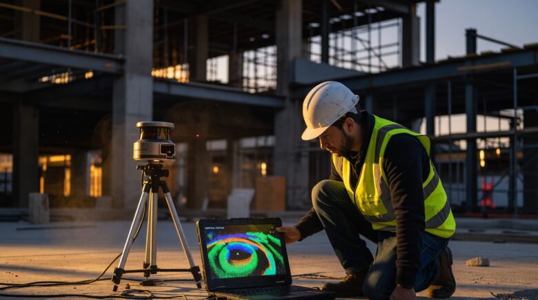
You’ve spent months calibrating your LiDAR system in the lab. The point clouds look immaculate. The range accuracy is within 2 centimeters. Then you bolt the sensor onto a real vehicle, deploy it in a parking garage, and watch the entire pipeline collapse — ghost returns everywhere, range degrading by 40%, and your object detection algorithm flagging concrete pillars as pedestrians. If this sounds familiar, you’re not alone. LiDAR sensor deployment in real-world environments exposes a brutal gap between controlled-environment performance and field-level reality that even experienced engineering teams routinely underestimate.
The financial stakes are staggering. A 2023 report from McKinsey estimated that autonomous vehicle programs have collectively burned through over $100 billion in investment with deployment timelines repeatedly pushed back — often due to sensor integration failures rather than algorithmic shortcomings. In industrial robotics, a single LiDAR-related downtime event on an automated warehouse line costs an average of $22,000 per hour in lost throughput, according to industry estimates from the Material Handling Institute. Across infrastructure monitoring, agriculture, and smart city programs, misdeployed LiDAR systems are quietly draining engineering budgets at scale.
This guide breaks down the five most consequential mistakes engineers make when deploying LiDAR sensors in real-world environments. You’ll get specific, field-tested guidance on environmental compensation, calibration protocols, data pipeline architecture, multi-sensor fusion pitfalls, and mounting decisions — with data, expert insight, and actionable steps to help you avoid costly rework.
Key Takeaways
- Poor environmental compensation causes up to 40% range degradation in rain, fog, or dust — directly undermining system safety margins.
- Miscalibrated extrinsic parameters between LiDAR and camera sensors introduce up to 15 cm of spatial offset, rendering sensor fusion unreliable at 30+ mph speeds.
- Inadequate thermal management reduces LiDAR lifespan by 30-50%, adding $8,000–$25,000 in unplanned replacement costs per unit per year.
- Engineers who skip vibration isolation during mounting report a 3x higher rate of mechanical drift, requiring recalibration every 2-4 weeks instead of every 3-6 months.
- Data pipeline bottlenecks from unprocessed high-density point clouds (up to 2.4 million points/second on 128-channel sensors) cause latency spikes exceeding 200ms — a critical failure threshold for real-time autonomy systems.
- Organizations that invest in pre-deployment site surveys reduce field troubleshooting costs by an average of 35%, recovering the survey cost within the first 90 days of operation.
In This Guide
- Mistake 1: Ignoring Environmental Interference
- Mistake 2: Treating Calibration as a One-Time Event
- Mistake 3: Underestimating Mounting and Placement Impact
- Mistake 4: Building an Undersized Data Pipeline
- Mistake 5: Botching Multi-Sensor Fusion Integration
- Why Pre-Deployment Site Surveys Are Non-Negotiable
- Thermal Management: The Silent System Killer
- Choosing the Right LiDAR Type for Your Environment
- Regulatory and Safety Compliance Considerations
- The True Cost of Getting LiDAR Deployment Wrong
Mistake 1: Ignoring Environmental Interference
Most LiDAR systems are validated against manufacturer spec sheets tested under ideal lab conditions — clear air, stable temperature, controlled surfaces. Real-world environments are none of those things. Engineers who don’t build explicit environmental compensation into their deployment architecture find themselves chasing phantom failures that the hardware spec never warned them about.
Atmospheric scattering is the most immediate culprit. When light rain, fog, or road dust enters the beam path, photons scatter before reaching the target and return false echoes. A study by the National Institute of Standards and Technology (NIST) found that at a rainfall rate of 25 mm/hour, common solid-state LiDAR units experienced a 30–45% reduction in effective detection range. That’s not a minor nuisance — it can collapse a 200-meter detection window down to 110 meters.
Rain, Fog, and Dust: Quantifying the Degradation
The physics of optical interference are unforgiving. Near-infrared wavelengths (905 nm, the most common in commercial LiDAR) scatter more aggressively in water droplets than 1550 nm systems, making wavelength selection a critical environmental decision rather than a marketing footnote.
Dust is frequently underestimated in industrial and agricultural deployments. Fine particulate matter (PM2.5 and PM10) creates a diffuse scattering layer that compounds over distance. Engineers deploying systems in quarry, mining, or grain-handling environments report point cloud quality degrading by 60% within 30 minutes of heavy dust activity.
At fog visibility levels of 50 meters (dense fog conditions), most 905 nm LiDAR sensors lose more than 70% of their rated range. Only 1550 nm systems maintain roughly 50% range performance under identical conditions.
Solar Interference and Saturation Events
Direct solar exposure is another underappreciated threat. When sensors face low-angle sunlight — particularly at dawn or dusk — the detector array can saturate, producing a “sun blindness” zone that eliminates returns for several degrees of field of view. This is a known failure mode in roadside infrastructure LiDAR monitoring where sensor orientation isn’t adjusted seasonally.
Engineering teams should model solar azimuth and elevation angles for the deployment site across all seasons before finalizing sensor orientation. A 15-degree azimuth adjustment at installation can prevent entire forward-facing detection zones from going dark during morning commute hours.
| Environmental Condition | 905 nm LiDAR Range Loss | 1550 nm LiDAR Range Loss |
|---|---|---|
| Light Rain (5 mm/hr) | 10–15% | 5–8% |
| Heavy Rain (25 mm/hr) | 30–45% | 15–22% |
| Dense Fog (50m visibility) | 70%+ | 45–55% |
| Heavy Dust (industrial) | 50–65% | 30–40% |
| Direct Sunlight (low angle) | Saturation risk | Lower saturation risk |
Mistake 2: Treating Calibration as a One-Time Event
There is a persistent and expensive myth in engineering teams: that LiDAR calibration is something you do once at commissioning, document in a configuration file, and never revisit. This assumption costs organizations tens of thousands of dollars annually in misattributed software bugs and phantom sensor errors that are actually calibration drift.
Intrinsic calibration (beam angle, timing offset, per-channel intensity correction) and extrinsic calibration (sensor pose relative to a reference frame or other sensors) both degrade over time. Mechanical vibration, thermal cycling, and physical shock from road surfaces or industrial equipment all induce micro-level shifts that accumulate into measurable spatial errors within weeks or months.
How Quickly Does Calibration Drift?
Research from Carnegie Mellon University’s Robotics Institute found that vehicle-mounted LiDAR units operating on standard road surfaces showed statistically significant extrinsic drift within 4–8 weeks of initial calibration, with positional offsets reaching 8–12 cm in yaw over a 3-month period. At highway speeds, a 10 cm spatial offset translates to a timing error of several milliseconds — enough to misclassify the lane position of adjacent vehicles.
In fixed-infrastructure applications (bridge monitoring, smart intersection sensors), calibration drift is slower but still consequential. Temperature swings of 30°C or more — common in outdoor environments between winter and summer — introduce bracket expansion that shifts sensor aim by 0.5–2 degrees. Over a 50-meter detection range, that represents 0.4–1.7 meters of positional error at the target plane.
Teams that implement automated monthly recalibration workflows report 67% fewer sensor-attributed software bug reports, according to data aggregated from autonomous vehicle testing programs at Tier 1 automotive suppliers.
Calibration Tools and Protocols Worth Using
Target-based calibration using retroreflective checkerboards remains the most reliable method for extrinsic LiDAR-to-camera calibration. Targetless methods (feature-based, motion-based) are improving rapidly and can be embedded in continuous self-calibration pipelines — but they require high-quality motion estimation from IMU or wheel odometry to produce reliable results.
Open-source tools like Autoware’s calibration utilities and Hesai’s proprietary calibration software provide structured workflows. The key discipline is scheduling: build recalibration intervals into your system’s maintenance calendar, not as a reactive response to anomalies. Treat calibration like firmware updates — expected, scheduled, and documented.
“Calibration decay is the single most common root cause we find when auditing failed autonomous system deployments. Teams spend months debugging their perception stack and never check whether their sensor poses are still valid. It’s a $200,000 mistake hiding behind a 2-hour calibration session.”
Mistake 3: Underestimating Mounting and Placement Impact
Where you mount a LiDAR sensor is as consequential as which sensor you choose. Engineers who optimize the hardware selection process and then bolt the unit onto the nearest convenient bracket are making a critical category error. Placement governs field of view, occlusion patterns, vibration exposure, thermal conditions, and ground plane coverage — simultaneously.
Vibration isolation is the most technically demanding aspect of mounting design. Vehicle-mounted sensors on commercial trucks experience broadband vibration from 5 Hz to over 200 Hz, with resonance peaks that can directly couple into the sensor’s spinning mechanism (in mechanical LiDAR) or induce micro-vibration in solid-state units that degrades beam accuracy. Engineers who skip isolation dampers report 3x higher recalibration frequency compared to teams that spec appropriate vibration mounts.
Height, Angle, and Occlusion Trade-offs
Mounting height determines ground plane coverage and near-field blind zone size. A LiDAR mounted at 1.9 meters (typical passenger vehicle roof height) produces a ground contact region starting at approximately 3–5 meters in front of the vehicle, depending on vertical field of view. Dropping that height to 0.9 meters (bumper or grille level) eliminates most of the near-field blind zone but introduces severe occlusion behind low obstacles and dramatically increases debris and splash exposure.
Tilt angle — the depression angle of the sensor relative to horizontal — shapes how efficiently the vertical channels cover the region of interest. For autonomous driving, most teams target a forward-biased tilt of 3–5 degrees downward. For infrastructure monitoring of a traffic intersection, an outward tilt of 15–25 degrees may be optimal. There is no universal answer; site-specific modeling is essential.

Mounting LiDAR sensors near heat exhaust vents, engine compartments, or metal surfaces with high thermal mass causes localized temperature gradients that accelerate calibration drift and can exceed the sensor’s operating temperature range — voiding manufacturer warranties and triggering premature failure.
Protective Housings and Ingress Protection
IP rating selection is frequently mishandled. Engineers often default to IP67 (dust-tight, immersion-resistant to 1 meter) for all outdoor deployments, but IP67 does not protect against high-pressure water jets — a routine occurrence in vehicle wash cycles, industrial cleaning, or coastal spray environments. IP69K is the appropriate rating for those scenarios.
Window material matters equally. Many OEM sensor windows are optimized for optical transmission at the cost of scratch resistance. In mining or agricultural environments, airborne particulates abrade unprotected windows within months, reducing transmission efficiency by 15–30%. Sapphire or hardened anti-reflective-coated windows add $200–$800 per unit but extend service life by 2–4x in abrasive environments.
| Mounting Position | Key Advantages | Primary Risks | Typical Use Case |
|---|---|---|---|
| Roof/Overhead | 360-degree FOV, minimal occlusion | Height clearance, aerodynamic drag, high vibration exposure | AV perception, city mapping |
| Front Bumper | Reduced near-field blind zone | Debris impact, splash, severe occlusion | Low-speed AGVs |
| Corner Pods | Wide lateral coverage | Complex wiring, vulnerability to impacts | Parking, maneuvering |
| Fixed Infrastructure Pole | Wide area coverage, no vibration | Weather exposure, vandalism, seasonal solar shifts | Smart intersections, traffic monitoring |
Mistake 4: Building an Undersized Data Pipeline
LiDAR sensor deployment doesn’t end at the hardware. The data pipeline — from raw point cloud ingestion through preprocessing, storage, and algorithm consumption — is where many technically sound hardware setups collapse in practice. Engineers often design pipelines for the average-case data rate, not the worst-case burst rate that occurs during complex scenes.
A single 128-channel mechanical LiDAR (such as the Velodyne Alpha Prime or Hesai QT128) generates approximately 2.4 million points per second at 10 Hz rotation. At 32 bytes per point (XYZ + intensity + ring ID + timestamp), that’s roughly 77 MB/second of raw data per sensor. Multi-sensor rigs running 3–5 units simultaneously generate 230–385 MB/second — sustained, every second of operation.
Latency Budgets and Real-Time Constraints
End-to-end latency from photon emission to processed output must stay under 100ms for most real-time autonomy applications, and under 50ms for high-speed highway scenarios. The pipeline budget breaks down roughly as: sensor processing (10–20ms), data transport via Ethernet (1–5ms), preprocessing — ground removal, voxel downsampling (10–30ms), and detection algorithm inference (20–60ms depending on hardware).
When preprocessing is not optimized — particularly when teams skip voxel downsampling and feed raw 2.4M-point clouds directly to neural networks — GPU inference time alone can spike to 150–200ms. That single oversight blows the entire latency budget and makes the system unsafe for real-world speed ranges. This is analogous to how engineers managing compute resources in edge computing architectures must balance processing locality with throughput — the same constraints apply at the sensor level.
Unoptimized LiDAR data pipelines running raw point clouds through GPU inference experience latency spikes of 200ms or more — four times the 50ms ceiling required for highway-speed autonomous operations.
Storage Architecture for Long-Duration Deployments
Infrastructure monitoring applications (bridge health, tunnel inspection, smart city) require long-duration data retention. Raw LiDAR logs at 77 MB/second generate 6.6 TB per day, per sensor. Teams that don’t implement point cloud compression (e.g., Draco, ZSTD-compressed PCD) and tiered storage architectures face storage cost overruns that derail project budgets within the first quarter of operation.
The right architecture separates hot storage (NVMe SSD for last 24–72 hours of data) from warm storage (high-density HDD arrays for 30–90 days) from cold archival (cloud object storage with lifecycle policies). Lossy compression at the cold tier — reducing to semantic labels and statistical summaries rather than raw points — can cut long-term storage costs by 85–92% without meaningful impact on historical analysis workflows.
Implement adaptive point cloud downsampling at the sensor driver level — not in post-processing. Reducing raw point density by 60% before data leaves the sensor processing unit cuts downstream pipeline load dramatically while preserving detection-critical geometric features.
Mistake 5: Botching Multi-Sensor Fusion Integration
LiDAR rarely operates alone. Modern perception systems combine LiDAR with cameras, RADAR, IMUs, and GPS — each with different coordinate frames, timestamps, and data rates. Sensor fusion errors are insidious because they manifest as seemingly random perception failures rather than obvious hardware faults, making root cause diagnosis extremely time-consuming.
The most common fusion failure is temporal misalignment. LiDAR generates data at 10–20 Hz. Cameras typically run at 30 Hz. RADAR at 12–15 Hz. GPS at 1–10 Hz. If timestamps across sensors are not synchronized to a common time source (typically GPS-derived PPS signals accurate to ±1 microsecond), object tracks built from fused data will contain systematic position errors proportional to object velocity and timestamp offset.
Spatial Calibration Errors in Fusion Pipelines
Extrinsic calibration between LiDAR and camera must be accurate to sub-centimeter level for reliable projection of LiDAR points onto camera image planes. A 2 cm translation error in the Z-axis (depth) between sensor frames produces a 2–8 pixel projection error at 10–40 meters range. At 50 meters, a poorly calibrated 1-degree rotation error translates to nearly 90 cm of lateral offset — making it impossible to accurately associate 3D LiDAR detections with 2D camera bounding boxes.
The upstream consequences of fusion errors propagate into tracking and prediction. If a pedestrian’s LiDAR centroid is systematically offset 50 cm from their camera bounding box centroid, tracking algorithms will either split them into two tracks or produce noisy velocity estimates. Both failure modes degrade downstream planning and control. This is a domain where the principles of AI-driven data synthesis are increasingly being applied — adaptive fusion algorithms can learn to compensate for small calibration residuals, but they cannot fix large systematic errors.
“The perception stack is only as good as its weakest calibration link. We’ve seen teams spend 18 months building world-class detection algorithms, only to have them perform worse than a simple camera system because their LiDAR-camera extrinsics were off by 3 centimeters and nobody caught it.”
RADAR-LiDAR Fusion: The Geometry Challenge
RADAR provides velocity (Doppler) data that LiDAR cannot produce natively. But RADAR’s angular resolution is poor — typically 1–5 degrees versus LiDAR’s 0.1–0.2 degrees. Naive fusion approaches that attempt to match RADAR detections to LiDAR clusters on spatial proximity alone produce excessive false associations in dense traffic, where multiple RADAR returns fall within a single LiDAR cluster’s spatial footprint.
The correct approach uses probabilistic association (JPDA, MHT, or deep learning-based methods) with gating regions that account for the full uncertainty ellipsoid of each sensor modality. Teams that skip probabilistic gating report 40–60% higher false association rates in validation testing — a problem that only worsens in complex real-world scenarios.
Why Pre-Deployment Site Surveys Are Non-Negotiable
Engineering teams under schedule pressure routinely skip formal pre-deployment site surveys, treating them as optional overhead. This is a costly error. A structured site survey — typically costing $5,000–$15,000 in engineering time — prevents field failures that routinely cost $50,000–$200,000 in rework, reconfiguration, and lost operational time.
A proper site survey quantifies: ambient electromagnetic interference (which affects sensor electronics and communication), surface reflectivity characteristics (which affect return intensity calibration), competing optical sources (other LiDAR systems, pulsed lighting, laser safety systems), and physical obstructions that create operational blind zones not visible in CAD models.
Reflectivity Mapping and Material Characterization
Retroreflective surfaces — road markings, safety vests, road signs — return 10–100x more intensity than typical diffuse surfaces. Without range intensity calibration, these surfaces trigger false maximum-range readings or detection confidence anomalies. Black surfaces (wet asphalt, carbon-fiber panels, certain tire compounds) are near-absorbers at 905 nm, sometimes returning fewer than 1% of emitted photons. This creates “invisible” zones in point clouds that must be explicitly mapped and handled by the perception stack.
In smart city and infrastructure deployments, interference from competing LiDAR units (crosstalk) is an emerging problem as sensor density increases. Two mechanically scanning LiDAR units within 50 meters of each other can inject inter-sensor returns that appear as valid detections. Frequency-hopping and coded pulse approaches from newer sensor generations address this, but only if engineering teams actually select and configure these modes — most default configurations don’t enable interference mitigation.
In dense urban intersections with 4+ LiDAR sensors deployed simultaneously, inter-sensor crosstalk can account for up to 12% of all detected points in shared field-of-view zones — without any filtering, that’s a 12% false positive floor in your perception system.
Thermal Management: The Silent System Killer
Operating temperature is one of the most thoroughly specified parameters in LiDAR datasheets and one of the most thoroughly ignored in deployment planning. Most commercial LiDAR sensors specify operating ranges of -10°C to +60°C. What datasheets often don’t communicate clearly is that sustained operation near the thermal ceiling degrades laser diode output power, increases dark current noise, and reduces detector sensitivity — degrading range performance well before triggering a thermal shutdown event.
Laser diode degradation follows the Arrhenius relationship: every 10°C increase in junction temperature approximately doubles the rate of electro-optical degradation. A sensor running at 55°C ambient (achievable in a sealed enclosure on a summer afternoon) ages its laser diodes roughly 8x faster than one running at 25°C. This translates directly to mean-time-to-failure: a sensor rated for 100,000 hours at 25°C may achieve fewer than 40,000 hours at 55°C.
Active vs Passive Thermal Management
Most OEM sensors use passive thermal management — heatsinks and thermal interface materials that rely on convective airflow. In sealed enclosures with no external airflow, this approach fails rapidly. Engineers deploying sensors in sealed roadside cabinets, vehicle trunk compartments, or industrial housings must add active thermal management: forced air cooling, thermoelectric coolers (TECs), or liquid cooling loops for high-power multi-sensor arrays.
The cost-benefit is clear. Active thermal management systems for a single-sensor installation run $300–$1,500. Premature sensor replacement due to thermal degradation costs $8,000–$25,000 per unit. Even a 20% reduction in thermal-related failures pays back a thermal management investment many times over within a 2-year deployment period.
| Thermal Management Approach | Cost per Sensor | Effective Temp Range | Best For |
|---|---|---|---|
| Passive Heatsink Only | $0 (built-in) | -10°C to +45°C | Open-air, well-ventilated mounts |
| Forced Air Cooling | $50–$300 | -20°C to +55°C | Vehicle rooftop, semi-enclosed housings |
| Thermoelectric Cooler (TEC) | $300–$800 | -30°C to +60°C | Sealed industrial enclosures |
| Liquid Cooling Loop | $800–$2,000 | -40°C to +70°C | High-density multi-sensor rigs |
Cold-climate deployments present an equal and opposite challenge. Below -20°C, sensor startup current spikes can damage motor drivers in spinning LiDAR designs, and condensation inside sensor housings (during warmup cycles) risks short-circuit damage. Heater elements integrated into sensor mounts — a $50–$200 addition — prevent both failure modes and are standard practice in Scandinavian and Canadian deployments.
Choosing the Right LiDAR Type for Your Environment
One of the foundational errors in LiDAR sensor deployment is treating sensor selection as a procurement exercise rather than an engineering decision. Different LiDAR architectures have fundamentally different strengths and failure modes. Matching architecture to deployment environment is prerequisite to everything else.
The three dominant architectures in field deployment today are: mechanical spinning LiDAR (360-degree coverage, highest point density, highest vibration sensitivity), solid-state LiDAR (no moving parts, limited field of view, better vibration tolerance, lower cost), and MEMS-based LiDAR (fast scan patterns, intermediate durability, emerging technology). A fourth category — flash LiDAR — is gaining ground in short-range industrial applications.
Architecture Decision Matrix
The choice is not purely technical. Total cost of ownership — factoring in mean time between failure, calibration maintenance cost, and replacement logistics — often favors lower-spec sensors with better durability over high-performance units that require frequent servicing. Just as organizations evaluating technology infrastructure investments must think beyond upfront cost (a principle well-illustrated in storage technology comparisons), LiDAR selection demands a lifecycle view.
| LiDAR Type | FOV | MTBF | Vibration Tolerance | Approx. Unit Cost |
|---|---|---|---|---|
| Mechanical Spinning | 360° horizontal | 50,000–80,000 hrs | Low — requires isolation | $2,000–$30,000 |
| Solid State (OPA/Flash) | 30°–120° limited | 100,000+ hrs | High — no moving parts | $500–$5,000 |
| MEMS-Based | 60°–120° | 80,000–100,000 hrs | Medium | $1,000–$8,000 |
| Flash LiDAR | Up to 120° | 100,000+ hrs | Very High | $300–$3,000 |
“Solid-state is not inherently better than spinning — it’s better for specific applications. Teams that default to solid-state for everything because it’s ‘the future’ are discovering that limited FOV forces them to use 4–6 sensors to cover what one 360-degree unit handles. The system cost and integration complexity multiplies, not decreases.”
Regulatory and Safety Compliance Considerations
LiDAR sensor deployment operates within a growing web of regulatory requirements that many engineering teams discover only after installation — triggering costly retrofits. Laser safety classification under IEC 60825-1 governs human exposure limits. Most commercial LiDAR systems are Class 1 (eye-safe under all intended operating conditions), but engineering teams that modify sensor operating parameters — increasing power for longer range — can inadvertently reclassify the device, requiring new safety assessments and restricted-access zones.
For vehicle-mounted deployments in the United States, FMVSS (Federal Motor Vehicle Safety Standards) compliance and in some states, specific autonomous vehicle testing permit requirements, govern what sensor configurations are legally permissible on public roads. In the European Union, the UNECE WP.29 framework for automated vehicle systems increasingly specifies sensor performance floor requirements that directly affect hardware selection decisions.
Data Privacy and Point Cloud Regulations
An emerging compliance burden is data privacy regulation applied to point cloud data. In jurisdictions with strict biometric data rules (GDPR in Europe, CCPA in California, BIPA in Illinois), pedestrian-resolution point clouds collected in public spaces may constitute biometric data if they can be used to uniquely identify individuals. Engineering teams deploying infrastructure LiDAR in smart city applications must implement anonymization pipelines — automated skeletal suppression, point cloud masking — before storing or transmitting pedestrian data.
Failure to implement compliant data handling can result in enforcement actions. The Illinois BIPA statute carries statutory damages of $1,000–$5,000 per violation per instance — a figure that scales catastrophically when a sensor logging 30 pedestrians per minute operates for months without compliant data practices. This intersection of data management and sensor deployment is an area where technology teams increasingly need cross-functional legal input from day one of deployment planning.
The True Cost of Getting LiDAR Deployment Wrong
Engineering managers often view LiDAR deployment errors as technical problems with technical solutions. They are that — but they are also financial events with compounding consequences that extend well beyond the immediate fix cost. Understanding the full cost structure changes how much pre-deployment investment is justifiable.
Direct costs of a failed deployment include: sensor replacement ($2,000–$30,000 per unit), engineering labor for root cause analysis and redesign (typically 200–500 hours at $150–$250/hour), and project schedule overruns that ripple into contract penalties or competitive displacement. Indirect costs — delayed product launches, customer confidence erosion, regulatory scrutiny triggered by safety incidents — are harder to quantify but routinely exceed direct costs by 3–5x.
According to analysis from the RAND Corporation, a single AV safety incident attributable to sensor failure can trigger regulatory review processes lasting 6–18 months, delaying entire program commercialization timelines and costing affected companies an average of $45–$120 million in market opportunity.
Building the Business Case for Rigorous Deployment Engineering
The return on investment for rigorous pre-deployment engineering is substantial and calculable. A team that invests $50,000 in proper site surveys, environmental testing, calibration infrastructure, and thermal management engineering across a 10-sensor deployment is protecting against an expected failure cost profile of $200,000–$800,000 based on industry failure rate data. That’s a 4:1 to 16:1 expected return on prevention investment.
The analogy to other technology investment decisions is direct. Just as wearable technology deployments require upfront integration rigor to deliver reliable health data (as explored in our coverage of wearable technology in health tracking), LiDAR systems require the same engineering discipline to deliver on their promise. The hardware is only the beginning of the value chain. The deployment architecture is where that value is either captured or squandered.
Organizations that implement structured LiDAR deployment engineering programs — including pre-deployment surveys, scheduled calibration, and thermal management — report 42% lower total 3-year cost of ownership compared to teams that treat deployment as a plug-and-play exercise.
Real-World Example: Smart Intersection Deployment — Midwest Transportation Authority
In early 2022, a midwestern regional transportation authority deployed 12 LiDAR sensors across 3 signalized intersections as part of a federally funded smart city pilot. The $1.8 million deployment used 32-channel mechanical LiDAR units mounted on existing signal poles at 5.2 meters height. Within 6 weeks, the operations team began reporting erratic vehicle detection performance — particularly during morning rush hours between 7:00 and 9:00 AM. Detection accuracy dropped from a validated 94% in commissioning testing to 71% in live traffic, with a disproportionate failure rate at two specific intersections facing east.
A post-mortem engineering audit — costing $28,000 in consulting fees — identified three compounding failures. First, the east-facing sensors were experiencing solar saturation for 40–70 minutes each morning from October through March, creating a forward detection blackout during the highest-traffic period. Second, bracket thermal expansion during summer heat (ambient temperatures reaching 38°C inside the sealed pole-top housings) had shifted sensor aim by 1.8 degrees downward, shrinking the detection zone in front of pedestrian crosswalks by 4.2 meters. Third, calibration had not been revisited since commissioning, and 7 of the 12 units showed extrinsic drift exceeding 8 cm. The combined effect produced the observed 23-percentage-point accuracy drop.
Remediation required $156,000 in engineering labor, bracket replacement, active cooling unit installation, and full recalibration across all 12 sensors. The authority also implemented a rotating calibration schedule (every 8 weeks), installed temperature-controlled enclosures ($4,200 per pole), and reoriented the two east-facing sensors by 12 degrees azimuth to avoid direct solar exposure during peak hours. Total remediation cost: $189,000 — more than 10% of the original deployment budget.
Following remediation, detection accuracy recovered to 96.3% — exceeding the original commissioning benchmark. More significantly, the authority used the experience to develop a 47-page deployment engineering standard that is now applied to all subsequent sensor installations. Their estimated cost avoidance from applying this standard to a follow-on 28-sensor expansion project was $340,000 — nearly double the remediation cost that prompted it. The lesson: rigorous deployment engineering isn’t a cost center. It’s the highest-ROI investment in any sensor program.
Your Action Plan
-
Conduct a formal pre-deployment site survey before any hardware procurement
Document ambient electromagnetic interference, surface reflectivity profiles, competing optical sources, and seasonal solar azimuth/elevation angles. Invest $5,000–$15,000 in this phase — it prevents 10–20x that cost in field rework. Include thermal modeling of intended enclosures under peak summer and minimum winter ambient temperatures.
-
Select LiDAR architecture based on deployment environment — not on marketing recency
Map your requirements (FOV, range, vibration environment, IP rating, temperature range) against the architectural trade-off table. Calculate total 3-year cost of ownership — including calibration labor, replacement likelihood, and thermal management — not just unit price. Require factory acceptance testing data for every unit received.
-
Design vibration isolation and thermal management into the mounting system from day one
Specify isolation mounts rated for your deployment vehicle or structure’s vibration PSD spectrum. Add active thermal management for any sealed enclosure where ambient exceeds 40°C. Budget $300–$2,000 per sensor position for this — it extends sensor life by 2–4x and reduces calibration drift frequency by 50–70%.
-
Implement a synchronized multi-sensor time architecture before writing any fusion code
Deploy a GPS-disciplined PPS time source (or IEEE 1588 PTP network time protocol) providing sub-microsecond timestamp accuracy across all sensors. Do not attempt to fuse LiDAR, camera, and RADAR data without hardware-level time synchronization. Temporal misalignment is the leading hidden cause of fusion system failures.
-
Build a calibration maintenance schedule into your operational plan — not your emergency response plan
Define calibration intervals based on your deployment’s vibration and thermal exposure: monthly for vehicle-mounted systems, quarterly for fixed infrastructure. Create standardized calibration procedures with acceptance criteria. Log all calibration events with before/after extrinsic parameters and track drift trends over time to predict when components need replacement.
-
Architect your data pipeline for worst-case throughput, not average-case
Measure peak point cloud density in your most complex operational scenarios (dense urban traffic, crowded warehouse aisles). Design your pipeline to handle 2x that peak without latency degradation. Implement adaptive downsampling at the driver level, tiered storage with compression, and end-to-end latency monitoring with automated alerting when pipeline latency exceeds 80% of your real-time threshold.
-
Address environmental compensation explicitly in your perception stack design
Implement dynamic range gating that adjusts detection thresholds based on atmospheric condition estimates (from onboard weather sensors or external API data). Build intensity normalization into your preprocessing pipeline to handle retroreflective and low-reflectivity surfaces. Test your system explicitly in rain, dust, and high solar incidence conditions before live deployment — not after.
-
Engage legal and compliance review on data privacy and laser safety before deployment
Confirm your sensor’s laser classification under IEC 60825-1 for your specific operating configuration. Map your data collection practices against applicable privacy regulations (GDPR, CCPA, BIPA) and implement anonymization pipelines for pedestrian data. Document compliance decisions — in regulatory review scenarios, documented intent matters as much as technical implementation.
Frequently Asked Questions
How often should LiDAR sensors be recalibrated in field deployments?
For vehicle-mounted systems on standard road surfaces, plan for recalibration every 4–8 weeks based on CMU research showing statistically significant drift in that window. For fixed infrastructure deployments with low vibration exposure but significant thermal cycling, quarterly recalibration is typically sufficient. Implement drift monitoring between scheduled calibrations — if you see systematic positional offsets growing in your tracked object data, that’s a leading indicator that early recalibration is needed.
What is the best LiDAR wavelength for outdoor deployments?
For long-range outdoor applications requiring performance in rain and fog, 1550 nm systems offer meaningful advantages — roughly half the range degradation of 905 nm systems in heavy precipitation. However, 1550 nm sensors are 3–8x more expensive than comparable 905 nm units and use InGaAs detectors that are more sensitive to temperature. For most budget-constrained programs in moderate climates, high-quality 905 nm systems with appropriate environmental compensation in software provide a better total value. The wavelength decision should be driven by your specific precipitation environment and budget, not by wavelength marketing.
Can LiDAR sensors interfere with each other when deployed in the same area?
Yes. Mechanical spinning LiDAR units using pulsed Time-of-Flight can receive returns from adjacent sensors operating in the same zone, generating false detections. This is called inter-sensor crosstalk. Newer sensor generations offer coded pulse or frequency-hopping modes that mitigate this significantly. In infrastructure deployments with multiple sensors at a single intersection, select sensors from manufacturers that explicitly offer and document interference mitigation modes — and enable those modes during configuration.
What IP rating do I need for outdoor LiDAR deployments?
IP67 (dust-tight, immersion-resistant) is the minimum for outdoor automotive and infrastructure deployments. If your deployment includes vehicle wash cycles, coastal spray, or industrial pressure washing, you need IP69K — which specifically certifies resistance to high-pressure, high-temperature water jets. IP67 and IP69K are not interchangeable. Note that some manufacturers rate only the sensor body to IP69K while the connector interface may be IP67 — verify the complete assembly rating, not just the sensor body.
How do I handle LiDAR performance degradation in snow and ice conditions?
Snow presents multiple challenges: falling snow creates false returns similar to rain, but accumulated snow on sensor windows is a more critical failure mode. Most deployments in cold climates use heated windows or housings to prevent snow accumulation. Sensor window heaters run at 5–15W and prevent the most damaging failure mode — complete window occlusion. In software, snow can be partially mitigated by filtering based on intensity thresholds (fresh snow is highly retroreflective) and dynamic clustering that ignores very small, spatially dispersed return clusters consistent with precipitation rather than solid objects.
What causes LiDAR to detect “ghost” objects that aren’t really there?
Ghost detections have several common sources: inter-sensor crosstalk (returns from adjacent LiDAR units), multipath reflections (the laser beam bouncing off a glass or mirror surface and returning an indirect echo), atmospheric scattering in rain or fog creating diffuse returns, and retroreflective surfaces like road signs or safety vests producing artificially high-confidence returns that the detector interprets as solid objects at incorrect ranges. Systematic ghost detection analysis — classifying ghosts by their spatial distribution and intensity signature — usually points clearly to the dominant cause in a given environment.
How much does a professional LiDAR deployment engineering audit cost?
Professional deployment audits from specialized consultancies range from $15,000–$80,000 depending on scope, number of sensors, and deployment complexity. For autonomous vehicle programs, audits involving full stack review (hardware, calibration, fusion, pipeline) typically run $40,000–$80,000 and take 4–8 weeks. For infrastructure deployments of 5–20 sensors, focused audits covering site survey, calibration review, and data pipeline analysis typically run $15,000–$35,000. Based on industry data, organizations recover audit costs through avoided rework within 60–120 days of deployment.
Is solid-state LiDAR always better for vibration-heavy environments?
Solid-state LiDAR (OPA, flash, or MEMS-based) eliminates the rotating motor assembly of mechanical LiDAR, making it inherently more vibration-tolerant. However, MEMS mirror-based solid-state designs still contain moving micro-mechanical elements that, while far less sensitive than spinning assemblies, can still exhibit performance degradation under sustained high-frequency vibration. True flash LiDAR — which has no scanning elements whatsoever — offers the highest vibration immunity. For extreme vibration environments (heavy construction equipment, rail vehicles, mining machinery), flash LiDAR’s shorter range is often an acceptable trade-off for its mechanical robustness.
How do I calculate the right number of LiDAR sensors for full coverage of my deployment area?
Start by mapping required coverage zones in your site’s CAD model, including all mandatory detection ranges and any safety-critical blind zone limits. Model each sensor’s FOV cone (horizontal and vertical) and identify occlusion-producing obstacles in the environment. Overlap design — where adjacent sensor FOVs share a 10–20% coverage zone — is recommended for redundancy. As a rough heuristic, fixed infrastructure deployments for intersection monitoring typically require 2–4 sensors per intersection. Autonomous vehicle platforms typically require 1 primary 360-degree unit plus 2–4 supplemental solid-state units for near-field and forward-long-range coverage. Budget 20–30% additional sensor count for redundancy coverage of critical zones.
What connectivity and communication standards should I use for LiDAR data transmission?
Gigabit Ethernet (GigE) is the dominant standard for point cloud data transmission from LiDAR to processing units, with most commercial sensors outputting UDP packet streams compliant with manufacturer-specific protocols or the emerging OpenLiDAR standard. For vehicle-mounted systems, automotive Ethernet (100BASE-T1 or 1000BASE-T1) enables single-pair unshielded wiring with lower weight. For infrastructure deployments over long distances (pole to central server room), fiber optic Ethernet eliminates electromagnetic interference and supports runs exceeding 100 meters without signal degradation. Wireless transmission of raw LiDAR point cloud data is generally impractical due to bandwidth requirements — transmit processed detections or semantic labels wirelessly, not raw points. Those interested in how next-generation wireless standards affect data-heavy sensor applications can explore 5G vs Wi-Fi 7 trade-offs for infrastructure connectivity planning.
Sources
- McKinsey & Company — Autonomous Driving’s Future: Convenient and Connected
- NIST — Autonomous Vehicle Technology Research and Standards
- RAND Corporation — Autonomous Vehicles Research and Analysis
- International Electrotechnical Commission — IEC 60825-1 Laser Safety Standard
- UNECE — World Forum for Harmonization of Vehicle Regulations (WP.29)
- Carnegie Mellon University Robotics Institute — Sensor Calibration Research
- SAE International — J3016 Taxonomy and Definitions for Automated Driving Systems
- Velodyne LiDAR — LiDAR Sensor Technology and Application Notes
- U.S. Department of Transportation — Automated Vehicle Data and Research
- IDC — Smart City Technology and Sensor Market Analysis
- Material Handling Institute — Automation and Robotics Industry Research
- Luminar Technologies — LiDAR Architecture and Performance Documentation
- ISO — ISO 26262 Functional Safety for Road Vehicles Standard
- Autoware Foundation — Open-Source Autonomous Driving Calibration Tools
- IAPP — U.S. State Biometric and Privacy Legislation Tracker